10 Quick Time-Saving Excel Shortcuts & Mouse Tricks.

The one thing marketers agree on is there isn't enough time in the day to accomplish everything. Often the best way to find more time is to save time.

Improving your Excel skills is a great place to begin to claw back a few minutes on every project, because Excel is a tool used by most of us on a regular basis. It has so many incredible capabilities that are not immediately apparent. Just finding one trick can save you minutes every day.

Excel Tip No. 1: Automatically SUM() with ALT + =

Quickly add an entire column or row by clicking in the first empty cell in the column. Then enter ALT + ‘=' (equals key) to add up the numbers in every cell above.

Excel Tip No. 2: Logic for Number Formatting Keyboard Shortcuts

At times keyboard shortcuts seem random, but there is logic behind them. Let's break an example down. To format a number as a currency the shortcut is CRTL + SHIFT + 4.

Both the SHIFT and 4 keys seem random, but they're intentionally used because SHIFT + 4 is the dollar sign ($). Therefore if we want to format as a currency, it's simply: CTRL + ‘$' (where the dollar sign is SHIFT + 4). The same is true for formatting a number as a percent.

Excel Tip No. 3: Display Formulas with CTRL + `

When you're troubleshooting misbehaving numbers first look at the formulas. Display the formula used in a cell by hitting just two keys: Ctrl + ` (known as the acute accent key) – this key is furthest to the left on the row with the number keys. When shifted it is the tilde (~).

Excel Tip No. 4: Jump to the Start or End of a Column Keyboard Shortcut

You are thousands of rows deep into your data set and need to get to the first or last cell. Scrolling is OK but the quickest way is to use the keyboard shortcut CTRL + ↑ to jump to the top cell, or CTRL + ↓ to drop to the last cell before an empty cell.

When you combine this shortcut with the SHIFT key, you'll select a continuous block of cells from your original starting point.

Excel Tip No. 5: Repeat a Formula to Multiple Cells

Never type out the same formula over and over in new cells again. This trick populates all of the cells in a column with the same formula, but adjusts to use the data specific to each row.

Create the formula you need in the first cell. Then move your cursor to the lower right corner of that cell and, when it turns into a plus sign, double click to copy that formula into the rest of the cells in that column. Each cell in the column will show the results of the formula using the data in that row.

Excel Tip No. 6: Add or Delete Columns Keyboard Shortcut

Managing columns and rows in your spreadsheet is an all-day task. Whether adding or deleting, you can save a little time when you use this keyboard shortcut. CTRL + ‘-‘ (minus key) will delete the column your cursor is in and CTRL + SHIFT + ‘=' (equal key) will add a new column. From an earlier tip, think about CTRL + ‘+' (plus sign).

Excel Tip No. 7: Adjust Width of One or Multiple Columns

It's easy to adjust a column to the width of its content and get rid of those useless ##### entries. Click on the column's header, move your cursor to the right side of the header and double click when it turns into a plus sign.

Excel Tip No. 8: Copy a Pattern of Numbers or Even Dates

Another amazing feature built into Excel is its ability to recognize a pattern in your data, and allow you to automatically copy it to other cells. Simply enter information in two rows which establish the pattern, highlight those rows and drag down for as many cells as you want to populate. This works with numbers, days of the week or months!

Excel Tip No. 9: Tab Between Worksheets

Jumping from worksheet to worksheet doesn't mean you have to move your hand off the keyboard with this cool shortcut. To change to the next worksheet to the right enter CTRL + PGDN. And conversely change to the worksheet to the left by entering CTRL + PGUP.

Excel Tip No. 10: Double Click Format Painter

Format Painter is a great tool which lets you duplicate a format in other cells with no more effort than a mouse click. Many Excel users (Outlook, Word and PowerPoint too) use this handy feature, but did you know you can double-click Format Painter to copy the format into multiple cells? It's quite a time-saver.

Using Loops In VBA In Microsoft Excel.

Why Loops?

The purpose of a loop in VBA is to get Excel torepeat a piece of code a certain number of times. How many times the code gets repeated can be specified as a fixed number (e.g. do this 10 times), or as a variable (e.g. do this for as many times as there are rows of data).Loops can be constructed many different ways to suit different circumstances. Often the same result can be obtained in different ways to suit your personal preferences. These exercises demonstrate a selection of different ways to use loops.There is two basic kinds of loops, both of which are demonstrated here:

• Do…Loop and
• For…Next loops.

The code to be repeated is placed between the key words.

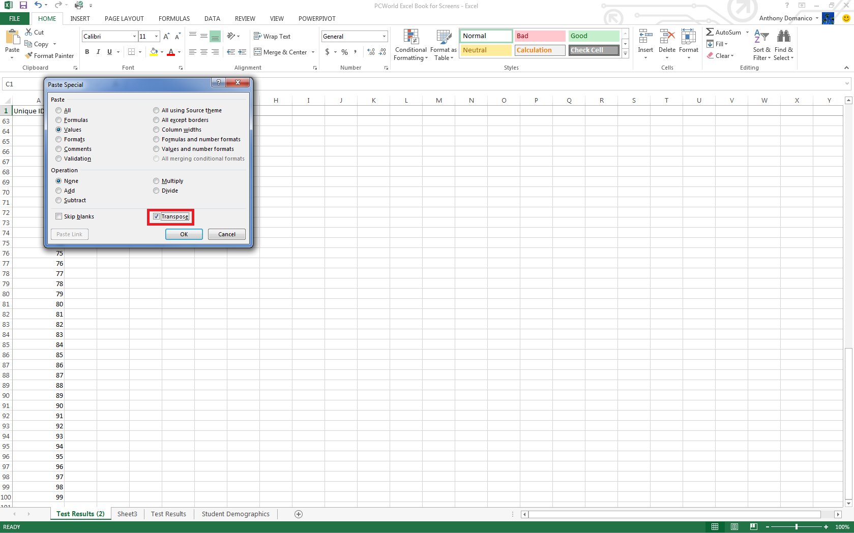
Open the workbook Using Loops in Visual Basic Application and take a look at the four worksheets. Each contains two columns of numbers (columns A and B). The requirement is to calculate an average for the numbers in each row using a VBA macro.

Now open the Visual Basic Editor (Alt+F11) and take a look at the code in Module1.  You will see a number of different macros. In the following exercises, first run the macro then come and read the code and figure out how it did what it did.

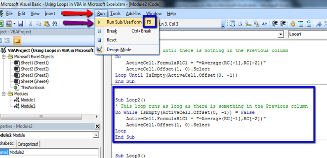
You can run the macros either from the Visual Basic Editor (VBE) by placing your cursor in the macro and pressing the F5 key, or from Excel by opening the Macros dialog box (ALT+F8) choosing the macro to run and clicking Run. It is best to run these macros from Visual Basic Editor by using Debug > Step Into (by pressing F8) so you can watch them as they work.

Instruction

If Developer Tab is not in the Ribbon..

• Open Excel.
• Go to VBA Editor (press Alt + F11)
• Go to Immediate Window. ( Ctrl + G)
• Write below Code.
  • Application.ShowDevTools = True

How to Insert VBA code in Excel

• Go to Developer Tab > Code Group > Visual Basic
• Click Insert > Module.
• Will open a Blank Module for you.
• Write / Paste provided code in that Module

How to Run VBA code in Excel

• Select anywhere in between the Code, Sub… End Sub
• Click Run & Run Sub or F5

Exercise 1: Do… Loop Until…

The object of this macro is to run down column C as far as is necessary putting a calculation in each cell as far as is Column B is filled or NotEmpty.

Select cell C2 before run the macro as macro is based on ActiveCell.

Here’s the code:

Sub Loop1()
'This loop runs until there is nothing in the Previous column
Do
ActiveCell.FormulaR1C1 = "=Average(RC[-1],RC[-2])"
ActiveCell.Offset(1, 0).Select
Loop Until IsEmpty(ActiveCell.Offset(0, -1))
End Sub

This macro places a formula into the active cell, and moves into the next cell down. It uses LoopUntil to tell Excel to keep repeating the code until the cell in the adjacent column (column B) is empty. In other words, it will keep on repeating as long as there is something in column B.

=Average(RC[-1],RC[-2]) is same as =AVERAGE(B1,A1) with respect to C1,  in R1C1 style, it’s trying to say, that, go for average of One Column left (c-1) and Two Column left (C-2)’ s data.

    Delete the data from Column C and ready for the next exercise

Exercise 2: Do While… Loop

The object of this macro is to run down column C as far as is necessary putting a calculation in each cell as far as is necessary.

Select cell C2 before run the macro as macro is based on ActiveCell.

Sub Loop2()
'This loop runs as long as there is something in the Previous column
Do While IsEmpty(ActiveCell.Offset(0, -1)) = False
ActiveCell.FormulaR1C1 = "=Average(RC[-1],RC[-2])"
ActiveCell.Offset(1, 0).Select
Loop
End Sub

The function IsEmpty = False means “Is Not Empty”

This macro does the same job as the last one using the same parameters but simply expressing them in a different way. In previous code, we are first running the Do… Loop code, then checking if criteria matched or not, where,

In this code, we are first checking the condition, and if matched then we are running the Do… Loop.

It uses Loop Until to tell Excel to if adjacent column (column B) is not empty, then only repeat the code.

Delete the data from Column C and ready for the next exercise

Exercise 3: Do While Not… Loop

The object of this macro is to run down column C as far as is necessary putting a calculation in each cell as far as is necessary.

Select cell C2 before run the macro as macro is based on ActiveCell.

Here’s the code:

Sub Loop3()
'This loop runs as long as there is something in the Previous column
Do While Not IsEmpty(ActiveCell.Offset(0, -1))
ActiveCell.FormulaR1C1 = "=Average(RC[-1],RC[-2])"
ActiveCell.Offset(1, 0).Select
Loop
End Sub

This macro makes exactly the same decision as the last one but just expresses it in a different way. IsEmpty = False means the same as Not IsEmpty. Sometimes you can’t say what you want to say one way, so VBA often offers an alternative syntax.

IsEmpty(ActiveCell.Offset(0, -1)) = False & Not IsEmpty(ActiveCell.Offset(0, -1)), are same way to say, do the repeated task, until adjacent left cell is filled with something, or not Empty.

Delete the data from Column C and ready for the next exercise

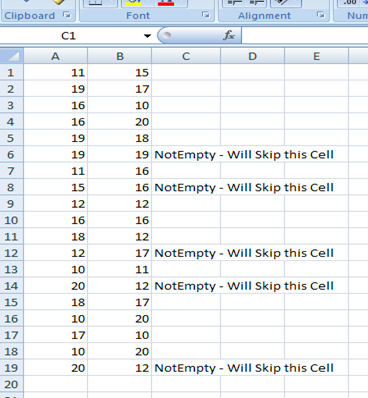
Exercise 4: Including an IF statement

The object of this macro is as before, but without replacing any data that may already be there.

Move to Sheet2, select cell C2 and run the macro Loop4.

Sub Loop4()
' This loop runs as long as there is something in the Previous column
' It does not calculate an average if there is already something in the cell
Do
If IsEmpty(ActiveCell) Then
ActiveCell.FormulaR1C1 = "=Average(RC[-1],RC[-2])"
End If
ActiveCell.Offset(1, 0).Select
Loop Until IsEmpty(ActiveCell.Offset(0, -1))
End Sub

The previous macros take no account of any possible contents that might already be in the cells into which it is placing the calculations. This macro uses an IF statement that tells Excel to write the calculation only if the cell is empty. This prevents any existing data from being overwritten.

The line telling Excel to move to the next cell is outside the IF statement because it has to do that anyway.

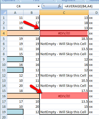
Exercise 5: Avoiding Errors

This macro takes the IF statement a stage further, and doesn’t try to calculate an average of cells that are empty.

First, look at the problem. Move to Sheet3, select cell C2 and run the macro Loop4.

Note that because some of the pairs of cells in columns A and B are empty, the =AVERAGE function throws up a #DIV/0 error (the Average function adds the numbers in the cells then divides by the number of numbers – if there aren’t any numbers it tries to divide by zero and you can’t do that!).

Sub Loop5()
' This loop runs as long as there is something in the NEXT column
' It does not calculate an average if there is already something in the cell
' nor if there is no data to average (to avoid #DIV/0 errors).
Do
If IsEmpty(ActiveCell) Then
If IsEmpty(ActiveCell.Offset(0, -1)) And IsEmpty(ActiveCell.Offset(0, -2)) Then
ActiveCell.Value = “”
Else
ActiveCell.FormulaR1C1 = "=Average(RC[-1],RC[-2])"
End If
End If
ActiveCell.Offset(1, 0).Select
Loop Until IsEmpty(ActiveCell.Offset(0, 1))
End Sub

Note that this time there are no error messages because Excel hasn’t tried to calculate averages of numbers that aren’t there, and criteria checking cell has been changed from adjacent column (B0 to adjacent Column D, as for testing purpose, we have change some of Cell in column B to Empty.

In this macro there is a second IF statement inside the one that tells Excel to do something only if the cell is empty. This second IF statement gives excel a choice. Instead of a simple If there is an If and an Else. Here’s how Excel reads its instructions…

“If the cell has already got something in, go to the next cell. But if the cell is empty, look at the corresponding cells in columns A an B and if they are both empty, write nothing (“”). Otherwise, write the formula in the cell. Then move on to the next cell.”

Exercise 6: For… Next Loop

If you know, or can get VBE to find out, how many times to repeat a block of code you can use aFor… Next loop.

select cell C2 and then run the macro Loop6.

Sub Loop6()
' This loop repeats for a fixed number of times determined by the number of rows
' in the range
Dim i As Long
lastcell = Range("A" & Cells.Rows.Count).End(xlUp).Row
For i = 0 To lastcell
ActiveCell.FormulaR1C1 = "=Average(RC[-1],RC[-2])"
ActiveCell.Offset(1, 0).Select
Next i
End Sub

This macro doesn’t make use of an adjacent column of cells like the previous ones have done to know when to stop looping. Instead it counts the number of rows in Column A and find the last filled cell by using below method.

Range(“A” & Cells.Rows.Count).End(xlUp).Row

That means, it goes to the last cell in A column (In case of Excel 2007 prior,  cells # A65536 ( 2^16), and for excel 2007 +  Cell Number A10485776 ( 2 ^ 20))  and then in come One Step Up, with pressing Control Key.. End(XlUp) and uses the For… Next method to tell Excel to loop that number of times.

In between any stage, if need to exit the loop, we can use EXIT FOR keyword to exit the FOR LOOP.

Exercise 7: Getting the Reference From Somewhere Else

In the above code we have checked Column A, to set the No Of Repeating Time,

 Range(“A” & Cells.Rows.Count).End(xlUp).Row

Instead of “A” we can use any other cell, to set the lastCell. By doing something like..

Range(“G” & Cells.Rows.Count).End(xlUp).Row

If you wanted to construct a loop that always ran a block of code a fixed number of times, you could simply use an expression like:

Instead of For i = 0 To LastCell , we can expression like of For i = 0 To 23. It will loop through Rows, and increase i form 0 to 23 / lastCell

Exercise 8: About Doing Calculations…

All the previous exercises have placed a calculation into a worksheet cell by actually writing a regular Excel function into the cell (and leaving it there) just as if you had typed it yourself. The syntax for this is:

ActiveCell.FormulaR1C1 = “TYPE YOUR FUNCTION HERE”

These macros have been using:

ActiveCell.FormulaR1C1 = “=Average(RC[-1],RC[-2])”

Because this method actuall change, just like regular functions – because they are regular functions. The calculating gets done in Excel because all that the macro did was to write the function.

If you prefer, you can get the macro to do the calculating and just write the result into the cell. VBA has its own set of functions, but unfortunately AVERAGE isn’t one of them. However, VBA does support many of the commoner Excel functions with its WorksheetFunction method.

On Sheet1 select cell C2 and run the macro Loop1.

Take a look at the cells you just filled in. Each one contains a function, written by the macro.

Now delete the contents from the cells C2:C20, select cell C2 and run the macro Loop8.

Here’s the code:

Sub Loop7()
Do
ActiveCell.Value = WorksheetFunction.Average(ActiveCell.Offset(0, -1).Value, _
ActiveCell.Offset(0, -2).Value)
ActiveCell.Offset(1, 0).Select
Loop Until IsEmpty(ActiveCell.Offset(0, -1))
End Sub

Take a look at the cells you just filled in. This time there’s no function, just the value. All the calculating was done by the macro which then wrote the value into the cell.

Real Excel Power Users Know These 11 Tricks.

There are two kinds of Microsoft Excel users in the world: Those who make neat little tables, and those who amaze their colleagues with sophisticated charts, data analysis, and seemingly magical formula and macro tricks. You, obviously, are one of the latter—or are you? Check our list of 11 essential Excel skills to prove it—or discreetly pick up any you might have missed.

Vlookup

Vlookup is the power tool every Excel user should know. It helps you herd data that's scattered across different sheets and workbooks and bring those sheets into a central location to create reports and summaries.

Vlookup helps you find information in large data tables such as inventory lists.

Say you work with products in a retail store. Each product typically has a unique inventory number. You can use that as your reference point for Vlookups. The Vlookup formula matches that ID to the corresponding ID in another sheet, so you can pull information like an item description, price, inventory levels, and other data points into your current workbook.

Summon the Vlookup formula in the formula menu and enter the cell that contains your reference number. Then enter the range of cells in the sheet or workbook from which you need to pull data, the column number for the data point you’re looking for, and either “True” (if you want the closest reference match) or “False” (if you require an exact match).

Creating charts

To create a chart, enter data into Excel with column headers, then select Insert > Chart > Chart Type. Excel 2013 even includes a Recommended Charts section with layouts based on the type of data you’re working with. Once the generic version of that chart is created, go to the Chart Tools menus to customize it. Don't be afraid to play around in here—there are a surprising number of options.

Excel 2013 includes Recommended Charts with layouts based on the type of data you're working with.

IF formulas

IF and IFERROR are the two most useful IF formulas in Excel. The IF formula lets you use conditional formulas that calculate one way when a certain thing is true, and another way when false. For example, you can identify students who scored 80 points or higher by having the cell report “Pass” if the score in column C is above 80, and “Fail” if it’s 79 or below.

IF formulas let you pull in just the data you need.

IFERROR is a variant of the IF Formula. It lets you return a certain value (or a blank value) if the formula you’re trying to use returns an error. If you’re doing a Vlookup to another sheet or table, for example, the IFERROR formula can render the field blank if the reference is not found.

PivotTables

PivotTables are essentially summary tables that let you count, average, sum, and perform other calculations according to the reference points you enter. Excel 2013 addedRecommended PivotTables, making it even easier to create a table that displays the data you need.

To create a PivotTable manually, ensure your data is titled appropriately, then go to Insert> PivotTable and select your data range. The top half of the right-hand-side bar that appears has all your available fields, and the bottom half is the area you use to generate the table.

PivotTables are a summarization tool that let you perform calculations according to the reference points you enter.

For example, to count the number of passes and fails, put your Pass/Fail column into theRow Labels tab, then again into the Values section of your PivotTable. It will usually default to the correct summary type (count, in this case), but you can choose among many other functions in the Values dropdown box. You can also create subtables that summarize data by category—for example, Pass/Fail numbers by gender.

PivotChart

Part PivotTable, part traditional Excel chart, a PivotChart lets you quickly and easily look at complex data sets in an easy-to-digest way. PivotCharts have many of the same functions as traditional charts, with data series, categories, and the like, but they add interactive filters so you can browse through data subsets.

PivotCharts help you easily digest complex data.

Excel 2013 added Recommended PivotCharts, which can be found under theRecommended Charts icon in the Charts area of the Insert tab. You can preview a chart by hovering your mouse over that option. You can also manually create a PivotChart by selecting the PivotChart icon on the Insert tab..

Flash Fill

Easily the best new feature in Excel 2013, Flash Fill solves one of the most frustrating problems of Excel: pulling needed pieces of information from a concatenated cell. When you’re working in a column with names in “Last, First” format, for example, you historically had to either type everything out manually or create an often-complicated workaround.

Flash Fill can automtically add data formatted the way you want without using formulas.

In Excel 2013, you can now just type the first name of the first person in a field immediately next to the one you’re working on, and click Home > Fill > Flash Fill, and Excel will automagically extract the first name from the remaining people in your table.

Quick Analysis

Excel 2013’s new Quick Analysis tool minimizes the time needed to create charts based on simple data sets. Once you have your data selected, an icon appears in the bottom right hand corner that, when clicked, brings up the Quick Analysis menu.

Quick Analysis speeds the process of working with simple data sets.

This menu provides tools like Formatting, Charts, Totals, Tables, and Sparklines. Hovering your mouse over each one generates a live preview.

Power View

Power View is an interactive data exploration and visualization tool that can pull and analyze large quantities of data from external data files. Go to Insert > Reports in Excel 2013.

Power View creates interactive, presentation-ready reports.

Reports created with Power View are presentation-ready with reading and full-screen presentation modes. You can even export an interactive version into PowerPoint. Several tutorials on Microsoft’s site will help you become an expert in no time.

Conditional Formatting

For most tables, Excel’s extensive conditional formatting functionality lets you easily identify data points of interest. Find this feature on the Home tab in the taskbar. Select the range of cells you want to format, then click the Conditional Formatting dropdown. The features you’ll use most often are in the Highlight Cells Rules submenu.

Conditional Formatting lets you easily highlight data points of interest.

For example, say you’re scoring tests for your students and want to highlight in red those whose scores dropped significantly. Using the Less Than conditional format, you can format cells that are less than -20 (a 20-point drop) with the Red Text or Light Red Fill with Dark Red Text function. You can create many different kinds of rules, with unlimited formats available via the custom format function within each item.

Transposing columns into rows (and vice versa)

Sometimes you’ll be working with data formatted in columns and you really need it to be in rows (or the other way around). Simply copy the row or column you’d like to transpose, right click on the destination cell and select Paste Special. A checkbox on the bottom of the resulting popup window is labeled Transpose. Check the box and click OK. Excel will do the rest.

The Paste Special feature transposes columns and rows.

Essential keyboard shortcuts

Keyboard shortcuts are the best way to navigate cells or enter formulas more quickly. We’ve listed our favorites below.

Control-Down/Up Arrow = Moves to the top or bottom cell of the current columnControl-Left/Right Arrow = Moves to the cell furthest left or right in the current row

Control-Shift-Down/Up Arrow = Selects all the cells above or below the current cell

Shift-F11 = Creates a new blank worksheet within your workbook

F2 = opens the cell for editing in the formula bar

Control-Home = Navigates to cell A1

Control-End = Navigates to the last cell that contains data

Alt-= = Autosums the cells above the current cell

Excel is arguably one of the best programs ever made, and it has remained the gold standard for nearly all businesses worldwide. But whether you’re a newbie or a power user, there's always something left to learn. Or do you think you've seen it all and done it all? Let us know what we've missed in the comments.

Speed up Firefox.

1. Speed up Firefox. If you have a broadband connection (and most of us do), you can use pipelining to speed up your page loads. This allows Firefox to load multiple things on a page at once, instead of one at a time (by default, it’s optimized for dialup connections). Here’s how:

Type “about:config” into the address bar and hit return. Type “network.http” in the filter field, and change the following settings (double-click on them to change them):
Set “network.http.pipelining” to “true”
Set “network.http.proxy.pipelining” to “true”
Set “network.http.pipelining.maxrequests” to a number like 30. This will allow it to make 30 requests at once.
Also, right-click anywhere and select New-> Integer. Name it “nglayout.initialpaint.delay” and set its value to “0?. This value is the amount of time the browser waits before it acts on information it receives.

2. Limit RAM usage. If Firefox takes up too much memory on your computer, you can limit the amount of RAM it is allowed to us. Again, go to about:config, filter “browser.cache” and select “browser.cache.disk.capacity”. It’s set to 50000, but you can lower it, depending on how much memory you have. Try 15000 if you have between 512MB and 1GB ram.

3. Reduce RAM usage further for when Firefox is minimized. This setting will move Firefox to your hard drive when you minimize it, taking up much less memory. And there is no noticeable difference in speed when you restore Firefox, so it’s definitely worth a go. Again, go to about:config, right-click anywhere and select New-> Boolean. Name it “config.trim_on_minimize” and set it to TRUE. You have to restart Firefox for these settings to take effect.

SMTP of Nepal ISPs.

Nepal telecommunication : smtp.ntc.net.np
WorldLink communications: smtp.wlink.com.np
Mercantile Communications: smtp.mos.com.np
Subisu Cablenet Pvt Ltd:  smtp.subisu.net.np
Websurfer :                       smtp.websurfer.com.np
Radius Communication:   smtp.radiusnp.com

Email Setting in Nepal according to ISP

World-link

Incoming Mail Server:   (POP3): pop3.wlink.com.np
Incoming Mail Server:   (IMAP): imap.wlink.com.np
Outgoing Mail Server:   (SMTP): smtp.wlink.com.np
Outgoing Mail Server:   (SSMTP): ssmtp.wlink.com.np (ssmtp port: 465)
Account name:             Your WorldLink username (the part before "@" on your e-mail address, for e.g.,                                           username is support for address support@wlink.com.np)
Password:                    Your account password.

Nepal Telecom's

Quick Configurations:
Presented below are the main configuration parameters for quick reference:
Incoming Mail Server Type: POP
Incoming Mail Server Address: pop3.ntc.net.np
Outgoing Mail Server Address:smtp.ntc.net.np
Incoming Mail Server Port:110
Outgoing Mail Server Port:25
Primary DNS:202.70.64.5
Gateway IP Address:202.70.64.10
Secondary DNS:202.70.64.15
Proxy Server Name:proxy.ntc.net.np
Proxy Server IP Address:202.70.64.15
Proxy Server Port:3128
Alternate Dial-in Numbers (except 15000):15050

Mercantile Communications

Incoming Mail Server (POP):       pop.mos.com.np 

Incoming Mail Server (IMAP):    imap.mos.com.np

Outgoing Mail Server:                  smtp.mos.com.np

Subisu Cablenet Pvt Ltd

Incoming Mail Server (POP):       pop.subisu.net.np 

Incoming Mail Server (IMAP):    imap.subisu.net.np

Outgoing Mail Server:                  smtp.subisu.net.np

Websurfer

1. Open Outlook. Select Account Settings... from the Tools menu.
   



2. On the E-mail tab, click New.
   



3. Select "Manually configure server settings or additional server types" and clickNext >. 
   


4. Select Email 
   


5. Enter the following information for E-mail Accounts. 
   
   • Your Name: Enter the name you wish recipients to see when they receive your message.
   • Email Address:This is the address that your contacts' email program will reply to your messages. This is also the address that will get recorded in your contacts' address book if they add you as a contact.
   • Account Type: POP3
   • Incoming mail server: Enter pop3.yourdomain.com
   • Outgoing mail server (SMTP): Enter smtp.websurfer.com.np
   • User Name: Enter your username
   • Password: If you wish for Outlook to save your password, check the box labeledRemember Password and enter your password in the text field.
   • Click More Settings...
 


6. Click on the Outgoing Server tab, and check out the box labeled My outgoing server (SMTP) requires authentication. Our SMTP server donot need authentication.
7. 
   
   


8. • Under Incoming Server (POP3), the port number should be set to 110.
   
9. Click Next.
10. Click Finish.

How to Clear Your Browser's Cache?

Your internet browser's cache stores certain information (snapshots) of webpages you visit on your computer or mobile device so that they'll load more quickly upon future visits and while navigating through websites that use the same images on multiple pages so that you do not download the same image multiple times. Occasionally, however your cache can prevent you from seeing updated content, or cause functional problems when stored content conflicts with live content. You can fix many browser problems simply by clearing your cache. This article contains instructions with screenshots on how to clear the cache for all major browsers.

If you are unsure of what browser version you are currently using, you can visit whatbrowser.org to find out.

Method 1 of 13: Chrome v10+

1. 
   1
   Open the settings on Chrome. Click the menu icon in the upper right corner of the browser to the right. Click settings on the bottom of the menu.
   • A faster way to get there is to press Control+Shift+Delete on a PC, or Shift+Command+Delete on a Mac.
2. 
   2
   From settings, click "Show advanced settings...". It's located at the very bottom of the settings section.
3. 
   3
   Scroll to the privacy section and click "Clear browsing data".
4. 
   4
   Select "Empty the cache". Uncheck all other options to avoid deleting browser history, cookies and other things you may wish to retain. Change "Obliterate the following items from" to "the beginning of time".
5. 
   5
   Press "Clear browsing data". You are done!

EditMethod 2 of 13: Chrome v1 - v9

1. 
   1
   Once your browser is open, select the Tools menu (the wrench in the upper-right corner) and select Options (Preferences on Mac).
2. 
   2
   On the Under the Hood tab, click the Clear Browsing data... button.
3. 3
   Select the Empty the cache check-box.
   
   
   
4. 4
   You can also choose the period of time you wish to delete cached information using the Clear data from this period dropdown menu.
   
   
   
5. 5
   Click the Clear Browsing Data button.
   
   
   

EditMethod 3 of 13: Safari for iOS, iPhone and iPad

1. 
   1
   Click on Settings from the home page.
2. 
   2
   Scroll down until you see "Safari." Click on it to bring up the option page.
3. 
   3
   Click "Clear Cookies and Data."A popup box will appear. Click "Clear Cookies and Data" again to confirm your choice.

EditMethod 4 of 13: Safari for Mac OS X

1. 
   1
   Once your browser is open, click the Safari menu and select Empty Cache...
2. 
   2
   Click Empty.

EditMethod 5 of 13: Safari for Windows

1. 
   1
   Once your browser is open, click the gear icon on the top right.
2. 
   2
   Select "Reset Safari..." This will prompt a screen to open.
3. 
   3
   Select "Remove all website data" at the very bottom of the prompt. Check or uncheck any other categories you want reset.
4. 
   4
   Click "Reset".

EditMethod 6 of 13: Internet Explorer 9 and 10

1. 
   1
   Once your browser is open, click the gear icon at the top right to open theSettings menu. Then, select Safety and Delete Browsing History....
   • Or, alternately, you may simply press Ctrl+Shift+Delete to open the Delete Browsing History window.
2. 
   2
   Select Temporary Internet Files. You will also need to uncheck all of the other boxes, especially Preserve Favorites website data. This option makes the window also delete objects from websites in your Favorites folder, which is necessary to completely clear your cache.
3. 
   3
   Click the Delete button near the bottom of the window to perform the operations (i.e. clear your cache by deleting temporary files).
4. 
   4
   Your computer will work for a moment, and then the process will be complete.You've successfully cleared Internet Explorer 9's Cache!

EditMethod 7 of 13: Internet Explorer 8

1. 
   1
   Once your browser is open, click the Tools menu. Or, optionally you may simply press Ctrl+Shift+Delete to open the Delete Browsing History window (and skip step 2)
2. 
   2
   Click on Delete Browsing History...
3. 
   3
   Select Temporary Internet Files.
4. 4
   Click the Delete button near the bottom of the window to delete your temporary files (i.e. clear your cache).
5. 
   5
   If you want the browser to automatically clear the cache whenever you close it, close the 'Delete Browsing History' window, select 'Internet Options' from the Tools menu, and check the 'Delete Browsing history on exit' checkbox.
   • Note: IE8 has a "feature" which retains some cookies even after you clear your cache if you do not UNCHECK the "Preserve Favorites Website Data." If you truly need to clear your cache, you will want to uncheck this!

EditMethod 8 of 13: Internet Explorer 7

1. 
   1
   Open IE 7 and click the Tools menu. Click the Delete Browsing History link at the top.
2. 
   2
   Under the Temporary Internet Files heading, click Delete files...
3. 3
   
   Click Yes when you see the prompt asking if you are sure you want to delete all temporary files.
4. 4
   Alternatively, clear your cache for just the current page you're visiting. Press and hold [Ctrl] on your keyboard, then Press [F5] or click on the Refresh button (square button on the toolbar with opposite-facing arrows).

EditMethod 9 of 13: Firefox

1. 
   1
   Go to "Clear Recent History":
   • On a PC, click the "Firefox" menu in the top left corner. Next, select the right arrow next to "History >", and click "Clear Recent History"
     • Or press Ctrl+Shift+Delete to open the recent history window.
   • On a Mac, from the Tools menu, select "Clear Recent History…"
     • Alternately, you can press Shift-Command-Delete.
2. 
   2
   Make sure "Details" is expanded, then select "Cache" from the list. Uncheck everything else.
3. 
   3
   In the "Time Range to Clear" drop down, select "Everything".
4. 
   4
   Select "Clear Now". Your computer will work for a moment, and the process will be complete. You've successfully cleared Firefox's Cache!

EditMethod 10 of 13: Android

1. 1
   Open the browser.
   
   
   
2. 
   2
   Hit the Menu Key.
3. 3
   Click on the "More Options" button.
   
   
   
4. 4
   Click on "Settings"
   
   
   
5. 5
   Hit "Clear Cache." You'll then be presented with a verification menu. Hit "Okay" or "Clear Cache" again (depending on the version of your phone) to complete the process.
   
   
   

EditMethod 11 of 13: Opera

1. 
   1
   Once your browser is open, select the "Settings" menu and click "Delete private data".
2. 
   2
   Make sure the "Delete entire cache" box is checked. Make sure any unwanted categories are left unchecked.
   • If you do not wish to delete cookies, saved passwords, etc., remove checks from them in the list.
3. 
   3
   Press "Delete".

EditMethod 12 of 13: Mozilla SeaMonkey

1. 
   1
   Once your browser is open, click the "Edit" menu and select "Preferences".
2. 
   2
   In the left-side list, open the "Advanced" node and select "Cache".
3. 
   3
   Click the "Clear Cache" button.